How to do common Excel and SQL tasks in Python

The code and data for this tutorial can be found in this Github repository. For more information on how to use Github, check out this guide. 

Data practitioners have many tools that they use to slice and dice data. Some people use Excel, some people use SQL — and some people use Python. The advantages of using Python are obvious when it comes to certain tasks. You can process much bigger datasets at much faster speeds. You can use open source machine learning libraries built on top of Python. You can easily import and export data in different formats. 

Python can become an essential part of any data analyst’s toolbox due to its versatility. However, it can be hard to get started. Most data analysts are probably familiar with either SQL or Excel. This tutorial is structured to help you transfer over skills and techniques from those two programs to Python.

First, let’s get you set up on Python. The easiest way to get started is to use Jupyter Notebook and Anaconda. This visual interface will allow you to plug Python code in and immediately see the output of your results. It’ll make it easy for you to follow along with the rest of this tutorial as well.

I highly recommend using Anaconda, but this beginners guide will also help you with installing Python directly — though that’ll make following this tutorial harder. 

Let’s start with the basics: opening up a dataset.

IMPORTING DATA

You can import .sql databases and process them in SQL queries. On Excel, you could double-click a file and then start working with it in spreadsheet mode. In Python, there’s slightly more complexity that comes at the benefit of being able to work with many different types of file formats and data sources.

Using Pandas, a data processing library, you can import a variety of file formats using the read function. A full list of the file formats you can import using this function is in the Pandas documentation. You can import everything from CSV and Excel files to the whole content of HTML files!

One of the biggest advantages of using Python is the ability to be able to source data from the vast confines of the web instead of only being able to access files you’ve downloaded manually. The Python requests library can help you sort through different websites and take data from them while the BeautifulSoup library can help you process and filter the data so you get exactly what you need. Be careful of usage rights issues if you’re going to go down this route.

(Don’t worry if you want to skip this part, you can! The raw csv file is here, and you can download it at will if you’d rather start this exercise without taking data from the web. Or you can git clone the entire repository.)

In this example, we’re going to take a Wikipedia table of countries by their nominal GDP per capita (a technical term that means an amount of income a country earns divided over the number of its population), and use the Pandas library in Python to sort through the data.

First, let’s import the different libraries we need. For more information on how imports work in Python, click here.

import pandas as pd
import numpy as np
import requests
from bs4 import BeautifulSoup
import re

We’ll need the Pandas library to process our data. We’ll need the numpy library to perform manipulations and transformations of numeric data. We’ll need the requests library to get HTML data from a website. We’ll need BeautifulSoup to process that data. Finally, we’ll need the regular expression library of Python (re) to change certain strings that will come up as we process the data. 

It’s not necessary to know much about regular expressions in Python, but they are a powerful tool you can use to match and replace certain strings or substrings. Here’s a tutorial if you wanted to learn more.

r = requests.get('https://en.wikipedia.org/wiki/List_of_countries_by_GDP_(nominal)_per_capita')

gdptable = r.text
soup = BeautifulSoup(gdptable, 'lxml')
table = soup.find('table', attrs = {"class" :"wikitable sortable"})

theads=[]
for tx in table.findAll('th'):
    theads.append(tx.text)

data =[]
for rows in table.findAll('tr'):
        row={}
        i=0
        for cell in rows.findAll('td'):
            row[theads[i]]=re.sub('\xa0', '',cell.text)
            i+=1
        if len(row)!=0:
            data.append(row)
print(data)

Credit to this website for some of the code.

Here’s a more technical explanation of how to grab HTML tables with Python code with more step-by-step instructions.

You can copy + paste the code above into your own Anaconda setup, and iterate with it if you want to play with some Python code!

The output from the code below, if you don’t modify it, is what is known as a list of dictionaries.

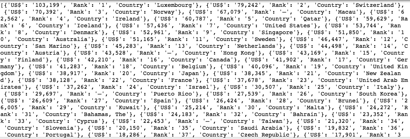
You’ll notice commas separating bracketed lists of key-value pairs. Each bracketed list represents a row in our dataframe, and each column is represented by the keys within: we are working with a country’s rank, its GDP per capita (expressed as US$), and its name (in ‘Country’).

For some more information on how data structures such as lists and dictionaries work in Python, this tutorial will help as well as this course: Intermediate Data Science Course by Springboard.

Thankfully, we don’t need to understand much of that in order to move this data into a Pandas dataframe, a similar way of aggregating data to a SQL table or an Excel spreadsheet. With one line of code, we’ve assigned and saved this data into a Pandas dataframe — as it turns out to be the case, lists of dictionaries are the perfect data format to be converted to a dataframe.

gdp = pd.DataFrame(data)

With this simple Python assignment to the variable gdp, we now have a dataframe we can open up and explore anytime we write out the word gdp. We can add Python functions to that word to create curated views of the data within. For a bit more of an in-depth look at what we just did with the equal sign and assignment in Python, this tutorial is helpful.

TAKING A QUICK LOOK AT THE DATA

Now, if we want to take a quick look at what we’ve done, we can use the head() function, which works very similarly to selecting a few rows in Excel or the LIMIT function in SQL. Use it handily to take a quick look at datasets without loading the whole thing! You can also insert a number within the head function if you want to look at a particular number of rows.

gdp.head()

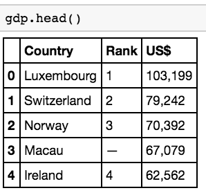
The output we get are the first five rows of the GDP per capita dataset (the default value of the head function), which we can see are neatly arranged into three columns as well as an index column. Be aware that Python starts indexes at 0 and not 1, such that if you wanted to call up the first value in a dataframe, you’d use 0 instead of 1! You can change the number of rows displayed by adding a number of your choice within the parentheses. Try it out!

RENAMING COLUMNS

One thing you’ll quickly realize in Python is that names with certain special characters (such as $) can become very annoying to handle. We’ll want to rename certain columns, something you can do easily in Excel by clicking on the column name and typing over the old name and something you can do in SQL either with the ALTER TABLE statement or sp_rename in SQL server.

In Pandas, the way to do it is with the rename function.

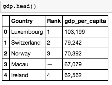
gdp = gdp.rename(columns = {'US$':'gdp_per_capita'}) 

In implementing the above function, we’ll be replacing the column header ‘US$’ with the column header ‘gdp_per_capita’. A quick .head() function call confirms that this change has been made.

DELETING COLUMNS

There’s been some data corruption! If you look at the Rank column, you’ll notice that there are random dashes scattered throughout it. That’s not good, and since the actual number order is disrupted, this makes the Rank column quite useless, especially with the numbered index column that Pandas gives you by default.

Fortunately, deleting a column is easy with a built-in Python function: del. By selecting columns through the use of square brackets appended to the dataframe name.

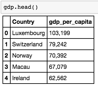
del gdp['Rank']

Now, with another call to the head function, we can confirm that the dataframe no longer contains a rank column.

CONVERTING DATA TYPES WITHIN COLUMNS

Sometimes, a given data type is hard to work with.This handy tutorial will break down the differences between the different data types in Python in case you need a refresher.

In Excel, you could right-click and find ways of converting columns of data to a different type of data quite easily. You could copy a set of cells rendered by formulas and paste special as values, and you can use formatting options to quickly switch between numbers, dates, and strings. 

It’s not as easy in Python to switch between one data type to the other sometimes, but it’s certainly possible.

Let’s first use the re library in Python. We will regular expressions to replace the commas within the gdp_per_capita column so we can more easily work with that column.

gdp['gdp_per_capita'] = gdp['gdp_per_capita'].apply(lambda x: re.sub(',','',x))

The re.sub function essentially takes every comma and replaces it with a blank space. This following tutorial goes into each function of the re library in detail.

Now that we’ve gotten rid of the commas, we can easily convert the column into a numeric one.

gdp['gdp_per_capita'] = gdp['gdp_per_capita'].apply(pd.to_numeric)

Now we can calculate a mean for the column.

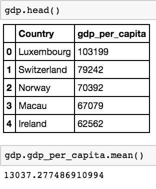
We can see that the mean of the GDP per capita column is about $13037.27, something we couldn’t do if the column were classified as strings (which you can’t perform arithmetic operations on). We can now do all sorts of calculations on the GDP per capita column that we weren’t able to do before — including filtering the columns by different values and determining what percentile rank values are for the column.   

SELECTING/FILTERING DATA

The basic need of any data analyst is to slice and dice a large dataset into actionable insights. In order to do that, you have to go through a subset of the data you have: this is where selecting and filtering data is very helpful. In SQL, this is accomplished with a mix of SELECT and different other functions, while in Excel, this can be done by dragging and dropping through data and implementing filters.

Using the Pandas library, you can quickly filter down with different functions or queries.

Let’s, as a quick proxy, only show countries that have a GDP per capita above $50,000.

This is how to do it:

gdp50000 = gdp[gdp['gdp_per_capita'] > 50000]

We assign a new dataframe with a filter that takes a column and creates a boolean variable — this function above essentially says “create a new dataframe for which there is a GDP per capita above 50000”. Now we can display gdp50000.

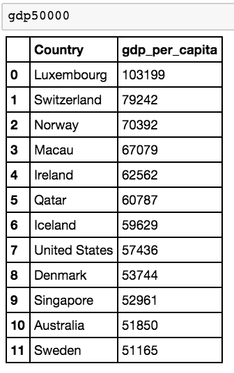
And now we see that there are 12 countries with a GDP above 50000!

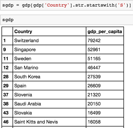
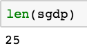
Now let’s select only rows that belong to a country that start with s.

We can now display a new dataframe containing only countries that start with s. A quick check with the len function (a life-saver for counting the number of rows in a dataframe!) indicates that we have 25 countries that fit the bill.

Now what if we want to chain those two filter conditions together?

Here’s where chained filtering comes in handy. You’ll want to understand how this works before filtering with multiple conditions. You’ll also want to understand the basic operators in Python. For the purposes of this exercise you just need to know that ‘&’ stands for AND — and that ‘ | ‘ stands for OR in Python. However, with a deeper understanding of all basic operators, you can easily manipulate data with all sorts of conditions. 

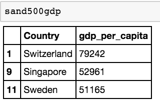
Let’s go ahead and work on filtering countries that both start with ‘S’ AND that have a GDP per capita above 50,000.

sand500gdp = gdp[(gdp.gdp_per_capita > 50000) & (gdp.Country.str.startswith('S'))]

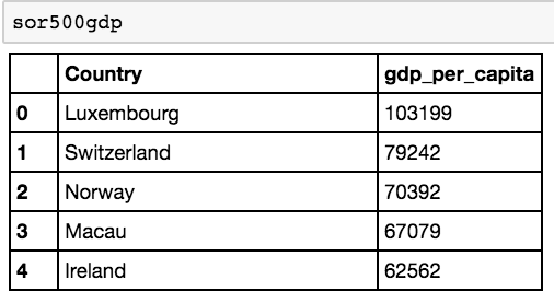
Now let’s work on those that start with S OR have over 50000 GDP per capita.

sor500gdp = gdp[(gdp.gdp_per_capita > 50000) | (gdp.Country.str.startswith('S'))]

There we go! We’re well on our way to working with filtered views in Pandas.

MANIPULATE DATA WITH CALCULATIONS

What would Excel be without functions that help you calculate different results?

Pandas in this case leans heavily on the numpy library and general Python syntax to put calculations together. We’re going to go through a simple series of calculations on the GDP dataset we’ve been working on. Let’s for example, calculate the sum total of all GDP per capita countries that are over 50,000.

gdp50000.gdp_per_capita.sum()

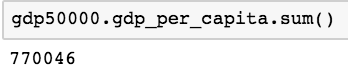
That’ll give you the answer of 770046. Using that same logic we can calculate all sorts of things — the full list can be located at the Pandas documentation under the computation/descriptive statistics section located on the menu bar at the left.

DATA VISUALIZATION (CHARTS/GRAPHS)

Data visualization is a very powerful tool — it allows you to share insights you’ve gained with others in an accessible format. A picture, after all, is worth a thousand words. SQL and Excel both have the capability to translate queries into charts and graphs. With the seaborn and matplotlib libraries, you can do the same with Python.

There are far more comprehensive tutorials on data visualization options — a favorite of mine is this Github readme document (all in text) which explains how to build probability distributions and a wide variety of plots in Seaborn. That should give you an idea of how powerful data visualization can be in Python. If you’re ever feeling overwhelmed, you can use a solution such as Plot.ly which might be more intuitive to grasp.

We’re not going to go through each and every data visualization option — suffice it to say that with Python, you’re going to have a lot more power to visualize things than anything SQL can offer, and you’ll have to trade-off the additional flexibility you gain with Python for how easy it is in Excel for generating charts from templates.

In this case, we’re going to build a simple histogram to show the distribution of GDP per capita for those countries that have more than $50,000 in GDP per capita.

gdp50000.hist() 

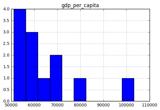
With this powerful histogram function (hist()) we can now generate a histogram that shows that most of the countries with a high GDP per capita cluster around the $50000 to $70000 range!

GROUPING AND JOINING DATA TOGETHER

Within Excel and SQL, powerful tools such as the JOIN function and pivot tables allow for the rapid aggregation of data.

Pandas and Python share many of the same functions that have been ported over from both SQL and Excel. You’ll be able to group data within datasets and join different datasets together. You can take a look here at the documentation. You’ll find that the join functionality offered by the merge function in Pandas is very similar to the one offered by SQL through the join command, while Pandas also offers pivot table functionality for those who are used to it in Excel.

We’re going to do a simple join here between the table we’ve developed with GDP per capita, and a list of world development indices from the World Bank.

Let’s first import the csv of country-level indicators.

country = pd.read_csv("Country.csv")

Let’s do a quick .head() function to take a look at the different columns in this dataset.

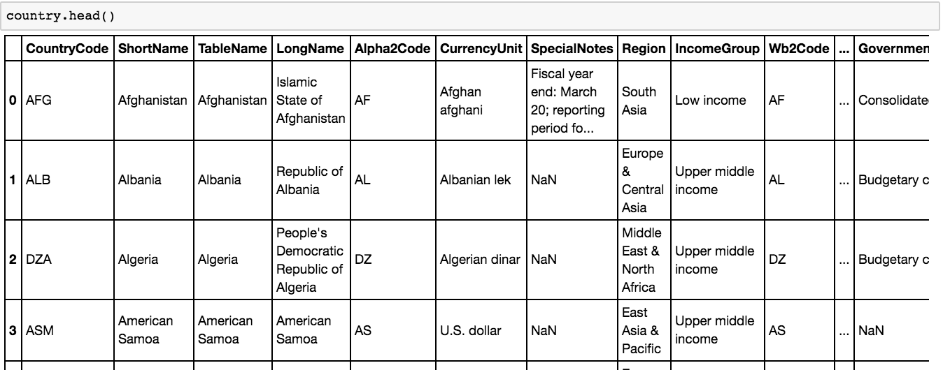
Now that we’re done, we can take a quick look and see that we’ve added a few columns that we can play with, including different years where data was sourced.

Now let’s merge the data:

gdpfinal = pd.merge(gdp,country, how = 'inner', left_on='Country', right_on = 'TableName')

We can now see the table incorporates elements of both our GDP per capita column and our new country-wide table with different data columns. For those familiar with SQL joins, you can see that we’re doing an inner join on the Country column of our original dataframe. 

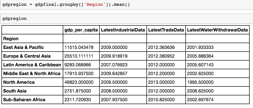
Now that we have a joined table, we may want to group countries and their GDP per capita by the region of the world they’re in.

We can now use the group by functions in Pandas to play around with the data grouped by region.

gdpregion = gdpfinal.groupby(['Region']).mean()

What if we want to see a permanent view of groupby summation? Groupby operations create a temporary object that can be manipulated, but they don’t create a permanent interface to aggregated results that can be built upon. For that, we’ll have to go through an old favorite of Excel users: the pivot table. Fortunately, pandas has a robust pivot table function.

gdppivot = gdpfinal.pivot_table(index=['Region'], margins=True, aggfunc=np.mean)

gdppivot

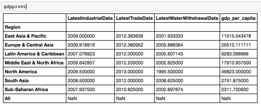
You’ll see we’ve picked up some extra columns we don’t need. Fortunately, with the drop function in Pandas, you can easily delete several columns.

gdppivot.drop(['LatestIndustrialData', 'LatestTradeData', 'LatestWaterWithdrawalData'], axis=1, inplace=True)

gdppivot

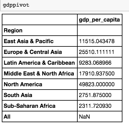
Now we can see that the GDP per capita differs depending on the regions in different parts of the world. We have a clean table with the data we want.

—

This is a very superficial analysis: you’d want to actually do a weighted mean since a GDP per capita for each nation is not representative of the GDP per capita of every nation in a group since populations differ across the nations within a group.

In fact, you’ll want to redo all of our calculations involving means to reflect a population column for each country! See if you can do that within the Python notebook you’ve just started. If you can figure it out, you’ll have been well on your way to transferring your SQL or Excel knowledge to Python. 

Got any comments or questions? Please leave them in the comments section on this blog post 🙂