RAPIDS is the new framework for distributed data science and machine learning provided by NVIDIA. You can use software optimized to do distributed work over GPU hardware rather than just standard CPU cores.

This provides a lot more computational speedup for machine learning training and tasks, with many people reporting speedups over large datasets and common machine learning tasks to the order of magnitude of 10x or 100x.

RAPIDS is actually a set of APIs in both Python and C++ to implement common machine learning tasks on GPUs instead of CPUs. It integrates with CUDA, which is a Nvidia framework for parallel computing. 

The purpose of this article is to build something like the Pandas Cookbook together for RAPIDS. I want to make it easy and intuitive to go from the Pandas and CPU ecosystem to taking advantage of GPUs and the increased computational power they can deliver.  

GPUs vs CPUs

GPUs are an odd product of the need for humans to game. Gaming is a computationally expensive activity. Tons of memory and processing needs to happen behind the scenes to simulate nearly real universes for gamers. 

This typically means that GPUs work with multiple cores (sometimes hundreds) that can perform simultaneous and parallel processing while CPUs are focused on a few threads with sequential calculations. While each individual thread may be slower than CPU threads, taken together on many shallow calculations, GPUs can vastly outperform CPUs by working on them all at once. There is some overhead on this, but on sufficiently large datasets or data pipelines, the differences lead to large speedups. 

Getting Access To GPUs or TPUs

Getting access to GPUs and TPUs can be quite difficult. TPUs are specific TensorFlow processing units. For GPUs, the options are to work with the cloud or to build your own GPU machine. 

On the cloud, there are several services that offer free GPU cloud hours, most prominently Kaggle and Google Colaboratory.

Google Colab offers the ability to use GPUs for free. However, the GPUs are randomly allocated and it’s hard to get good ones. The free one also cuts off after 12 hours. 

The pro version of Google Colab, at $9.99 a month, is available in the United States and offers premium availability for Nvidia GPUs. It also offers more uptime (up to 24 hours) and more lax restrictions when it comes to idle times. 

You can also create your own deep learning hardware. This tutorial shows you how to do it in under $1000, though it’ll require some setup and some patience on your side — though at the end, you’ll have a machine that will save you some variable cost. In practice, you’ll only want to do this if you’re serious about machine learning use cases, and using as much of the fixed cost compute as you can. 

Of course, if you use AWS, Microsoft Azure, or Google Cloud solutions, you can pay for GPU access on those platforms, though that may end up costing a lot.  

For the purposes of this playbook, we’re going to start using Kaggle, which comes with access to both TPUs and GPUs as accelerators, though you’ll need to verify a phone number to get access to that. Once you do, you can set up GPUs then install RAPIDS through the handy dataset. 

Then you can import datasets from Kaggle datasets and you’re off and running. However, Kaggle has a 41 hour weekly quota on GPU usage — which means that it’s ideal for short experiments and learning examples.

The Kaggle instance will pause every 40 minutes or so. The best practice would be to pause the instance and turn it off when you’re not using it.

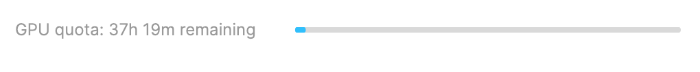
The above is a screenshot of my GPU usage. The usage will reset every week. You also won’t get access to the latest NVIDIA architecture, but it will be free. There’s an easy-to-access dashboard on your GPU and CPU usage as well. 

If you want to get started right away with powerful infrastructure, BlazingSQL offers a free hosted Jupyter environment with the latest version of the RAPIDS stack pre-installed and a bit of GPU memory to play with. They’re also offering beta access to clusters of cloud GPUs.

Rapids will be pre-installed, but it’ll be harder to get intuitive access to different datasets as you might on Kaggle — so we’ll stick with Kaggle for now for the importing data part. But BlazingSQL can be used in practice, especially since Kaggle’s data and compute limits are set more towards learning rather than production. 

cuDF’s role in Rapids

cuDF is meant to be the data manipulation layer of Rapids, allowing for the rapid manipulation of dataframes over GPUs. In the documentation, it describes cuDF as being useful for loading, joining, aggregating and filtering data.

You can think of it as a Pandas equivalent within Rapids and in fact many of the functions from cuDF map pretty closely to their Pandas equivalents.

In practice, when you’re dealing with data or wrangling data, you’re likely going to have to deal with cuDF if you want to work on RAPIDS on a GPU.

Dask-cuDF vs. cuDF vs. Pandas

Dask is a parallel processing library that slices up Pandas dataframes on CPUs. It can be used with cuDF combining multiple GPUs and chunking. This documentation from the RAPIDS team summarizes the difference and goes into detailed documentation of the different functions possible- from your standard filtering and value_counts() to more complex groupbys and aggregations.

The syntax here is very similar to Pandas — in practice, you’ll see using cuDF and Dask-cuDF as very similar experiences to the Pandas API, just with slightly less function completeness. 

It’s of course important to also note when it’s best to use each framework: 

• Dask-cuDF for when you have very large datasets that you need multiple GPUs to train on and you have more memory in your dataset than the GPU can handle 
• cuDF for when you have a large dataset that can be trained and wrangled on a single GPU and when you maybe don’t have access to multiple GPUs, such as our example on Kaggle, where you only have access to one GPU
• Pandas for a small enough dataset that can fit and be trained on CPU only. In practice, for most standard setups, unless you have a particularly strong computer with a GPU installed, Pandas will be “good enough” for now, especially with smaller datasets.

Dask-cuDF, cuDF Import/Export Data With Pandas and CSV

It’s relatively simple to go from different datatypes into the three frameworks, and pass dataframes from framework to framework. Let’s discuss how to transfer between the different frameworks.

It’s quite simple to go from a Pandas dataframe to a cuDF dataframe: it’s a one-line command. In this case, we take our predefined dataframe (seattlelibrarydf) of the Seattle Library inventory and convert it into a cuDF dataframe with many of the same properties (seattlelibrarycudf). 

This simple function helps turn a Pandas Dataframe into the cuDF equivalent. 

Common Functions

It’s time to put cuDF to the test and actually get working on a large dataset. In the case of Kaggle, we’re going to work with the Seattle Public Library dataset, a large collection of CSV files that tabulate the inventory of the Seattle Public Library as well as a set of CSVs that describe the yearly checkout patterns. Specifically, we’re going to join together the yearly checkout data and then do analysis on the inventory.

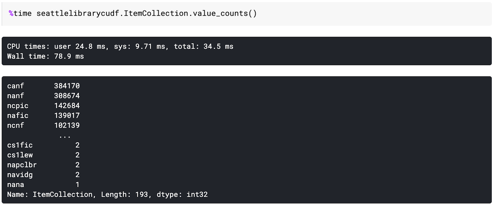
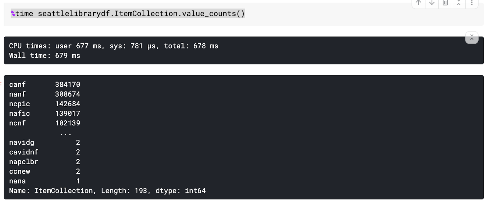
Let’s now look at a common function, the ubiquitous value_counts in Pandas. This takes a column and returns an aggregated count of cell values. In this case, we’ll do it on the different collection codes we can later join onto descriptions of the categories.

Note here that the syntax for the function in both Pandas and cuDF is essentially the same — but by using cuDF on an average-power GPU and a slightly larger than 1 GB dataset, with more than 2.5 million records, we achieve about a 10x speedup even in pre-processing the data, from 679 milliseconds to 78.9 milliseconds. 

Groupby/Aggregations

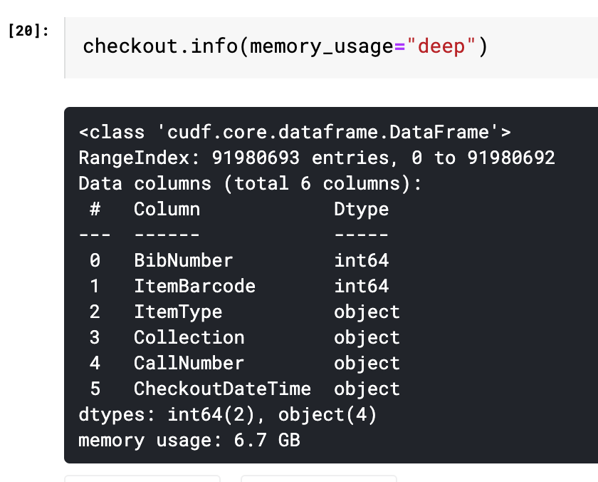
Now let’s get to the meat of the dataset and join together different datasets that form the yearly check-ins per each item. This is not a trivial exercise. By the end, we’ll have combined together a large dataset of multiple GB (about 7 gb, or slightly under 50% of the GPU memory allocation Kaggle gives us) with about 90 million rows. 

The read_csv function of cudf will also have some issues, specifically with the datatypes you need to define and validate. It will sometimes take columns and mix up datatypes, meaning you have to set them manually with the dtype variable.

However, cuDF is decently finicky about how you do this. So far, I’ve found that ‘int64’, ‘timestamp’, and ‘str’ (and it’s important that they be passed as strings) works, unlike the numpy variants suggested in the basic documentation. You can track the progress on this open Github issue. 

Let’s now do some data wrangling and joins. We want to see what ten items are most frequently checked out in the dataset. We can do this really quickly by slicing a value_counts() method call just like you might do in Pandas.  We’ll do this on the BibNumber column which serves as a primary key that unites both checkout data and the underlying information about each inventory item. 

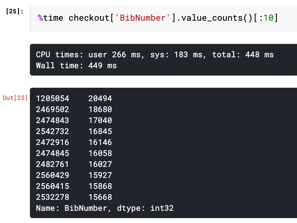
We get a bunch of item numbers. But what are the actual items here? Who are the authors? Can we say anything about these items beyond their key numbers.

To find that insight, we’ll have to perform a join of both the inventory information and the aggregated checkout data — and we’ll have to clean up the dates and times represented in the last CheckoutDateTime column.  This is something we may cover in another tutorial. 

For now, hopefully, you’ve learned enough to get set up on RAPIDS and CUDF and why you might want to use it.